Telco Customer Churn Analysis


import pandas as pd
import sklearn as sk

df = pd.read_csv("WA_Fn-UseC_-Telco-Customer-Churn.csv")
print(df.head())
df.T
print(df.dtypes)

#We try to predict whether customers will leave the service.
#Today, the fact that companies make a discount is to determine the possibility of the customer to leave.
#The Columns Except Churn -- Attribute
#Churn -- Target
#SeniorCitizen -- int64 -- Actually, True is expressed as 0 and 1 for False,
but it's not a problem since it's a single column.
#TotalCharges -- object -- It should have been a number, but it counted as text because of the comma!

df.TotalCharges = pd.to_numeric(df.TotalCharges, errors="coerce")
print(df.dtypes)
print(df.isnull().sum())
df.TotalCharges = df.TotalCharges.fillna(0)
print(df.isnull().sum())
df.columns = df.columns.str.lower().str.replace(" ","_")

string_columns = list(df.dtypes[df.dtypes=="object"].index)
for col in string_columns:
df[col]=df[col].str.lower().str.replace(" ","_")
print(df.head())
df.churn = (df.churn == "yes").astype(int)

from sklearn.model_selection import train_test_split
df_train_full, df_test = train_test_split(df,train_size=0.8,random_state=42)
df_train, df_val = train_test_split(df_train_full,train_size=0.75,random_state=42)
y_train = df_train.churn.values
y_val = df_val.churn.values
del df_train["churn"]
del df_val["churn"]

categorical = ["gender","seniorcitizen","partner","dependents", "phoneservice", "multiplelines", "internetservice", "onlinesecurity", "onlinebackup", "deviceprotection", "techsupport", "streamingtv", "streamingmovies","contract", "paperlessbilling", "paymentmethod"]
numerical = ["tenure","monthlycharges","totalcharges"]
train_dict = df_train[categorical+numerical].to_dict(orient="records")
print(train_dict[:1])

from sklearn.feature_extraction import DictVectorizer
dv = DictVectorizer(sparse=False)
dv.fit(train_dict)
X_train = dv.transform(train_dict)

from sklearn.linear_model import LogisticRegression
model = LogisticRegression(solver="liblinear",random_state=42)
model.fit(X_train, y_train)
val_dict = df_train[categorical+numerical].to_dict(orient="records")
X_val = dv.transform(val_dict)
y_pred = model.predict_proba(X_val)
print(model.score(X_train,y_train))
print(model.intercept_[0])
#print(dict(zip(dv.get_features_names_out(),model.coef_[0].
round(3))))
Forbes 2022 Billionaries Analysis


#Forbes 2022 Dataset

import pandas as pd

df=pd.read_csv("forbes_2022_billionaires.csv")
print(df.head())

#We have to remove letters and signs. We need to apply transform to
columns that should be numeric.

print(df.columns)
#Some column names have spaces, we have to fill those spaces with _.
#df.columns=df.columns.str.replace(" ","_")
print(df.columns)

print(df.shape)
#Row -- Sample
#Column -- Attribute
#print(df.dtypes)
#The Object data type must be converted to a numeric data type.

#print(df.isnull().sum())
#There is too much missing data in the Rating column.

import seaborn as sns
import matplotlib.pyplot as plt
import warnings
warnings.filterwarnings("ignore")

sns.set_theme()
sns.set(rc={"figure.dpi":90,"figure.figsize":(12,9)})
#sns.heatmap(df.isnull(),cbar=False)
#print(plt.show())

#Since removing missing data will result in loss of information,
we will replace them with the medians of the data set.

#rating_median=df["Rating"].median()
#print(rating_median)
#df["Rating"].fillna(rating_median,inplace=True)
#Since the number of other missing data is low, we removed it directly.
#df.dropna(inplace=True)
#print(df.isnull().sum().sum())
#print(df.info)

#Now object -- int64
#df["Reviews"].describe()
#df["Reviews"]=df["Reviews"].astype("int64")
#df["Reviews"].describe().round()
#We did the rounding.

#Now we will remove the letters M and K.
#df["Size"].replace("M","",regex=True,inplace=True)
#df["Size"].replace("k","",regex=True,inplace=True)
#df["Size"].unique()
#There is one column with text.
#size_median=df[df["Size"]!="Varies with device"]["Size"].astype(float).median()
#df["Size"].replace("Varies with device",size_median,inplace=True)
#df.Size=pd.to_numeric(df.Size)
#print(df.Size.head())
#df.Size.describe().round()

#Now let's remove the + and , signs. Then let's convert it to an int value.
#df.Installs=df.Installs.apply(lambda x:x.replace("+",""))
#df.Installs=df.Installs.apply(lambda x:x.replace(",",""))
#df.Installs=df.Installs.apply(lambda x:int(x))
#df.Installs.unique()

#Now let's remove the $ symbol.
#df.Price=df.Price.apply(lambda x:x.replace("$",""))
#df.Price=df.Price.apply(lambda x:float(x))
#df.Price.unique()

#Now ; Let's uncheck it. Next, let's separate the attributes, Type and Field.
#df.Genres=df.Genres.str.split(";").str[0]
#df.Genres.unique()
#Let's combine Music and MusicAudio genres.
#df.Genres.replace("Music Audio","Music",inplace=True)

#df.Last_Updated=pd.to_datetime(df.Last_Updated)

#Now we move on to the data visualization phase.
#df["Type"].value_counts().plot(kind="bar",color="blue")
#print(plt.show())
#We have seen that the number of free applications is more than
the number of paid applications.
#sns.boxplot(x="Type",y="Rating",data=df)
#print(plt.show())

#sns.countplot(y="Content_Rating",data=df)
#plt.title("Content rating with their counts")
#print(plt.show())

#sns.boxplot(x="Content_Rating",y="Rating",data=df)
#print(plt.show())

#cat_num=df["Category"].value_counts()
#sns.barplot(x=cat_num,y=cat_num.index,data=df)
#plt.title("The number of categories")
#print(plt.show())

#sns.scatterplot(data=df,y="Category",x="Price")
#print(plt.show())

#sns.histplot(df["Rating"],kde=True)
#print(plt.show())

#########################################

#We select the columns we are working on.

df=df.loc[:,["rank","personName","age","finalWorth","category","country",
"gender"]]
print(df.head())

df=df.rename(columns={"rank":"Rank","personName":"Name","age":"Age","finalWorth":
"TotalWorth","category":"Category","country":
"Country","gender":"Gender"})
print(df.head())

#Since the Rank column starts from 1 and progresses increasing,
we can accept it as an index column.
df=df.set_index("Rank")
print(df.head())

print(df.dtypes)
print(df.isnull().sum())
df.dropna(inplace=True)

#Data preprocessing is finished. Now we will extract the information.
print(df["Gender"].value_counts(normalize=True))
print(df[df["Country"]=="Turkey"].Gender.value_counts())

df_gender=df.groupby(["Gender"])
df_gender.Age.mean()

df_gender.size().plot(kind="bar")
sns.barplot(x=df.TotalWorth[:10],y=df.Name[:10])

df_country=df.groupby("Country")
df_country_count=pd.DataFrame(df._country.size().
sort_values(ascending=False),columns=["Counts"])
sns.barplot(x=df_country_count["Counts"][:10],y=df_country_count.index[:10])

House Prices Analysis


import pandas as pd
import sklearn as sk
import math

df_train = pd.read_csv("train.csv")
df_test = pd.read_csv("test.csv")

df_train.set_index("Id",inplace=True)
df_test.set_index("Id",inplace=True)

print(df_train.dtypes)
print(df_test.dtypes)

print("Train shape: ",df_train.shape)
print("Test shape: ",df_test.shape)

#Let's remove the columns with missing data.

cols_with_null = df_train.isnull().sum().sort_values(ascending=False)
cols_to_drop = (cols_with_null.head(6).index).to_list()
print(cols_to_drop)

df_train.drop(cols_to_drop,axis=1,inplace=True)
df_test.drop(cols_to_drop,axis=1,inplace=True)

df_train.describe().T

y = df_train.SalePrice
X = df_train.drop(["SalePrice"],axis=1)

from sklearn.model_selection import train_test_split

X_train, X_val, y_train, y_val = train_test_split(X,y,train_size=0.95,random_state=0)

categorical_cols = [cname for cname in X_train.columns
if X_train[cname].nunique()leesthan10 and X_train[cname].dtype="object"]
print(len(categorical_cols))

numerical_cols = [cname for cname in X_train.columns
if X_train[cname].dtype in [int64,float64]]

my_cols=categorical_cols+numerical_cols

X_train=X_train[my_cols]
X_val=X_val[my_cols]
X_test=df_test[my_cols]

from sklearn.pipeline import Pipeline
from sklearn.impute import SimpleImputer
from sklearn.preprocessing import StandardScaler
from sklearn.preprocessing import OneHotEncoder

numerical_transformer = Pipelinesteps[
(imputer_num, SimpleImputer(strategy="median")),
(scaler, StandardScaler())
]

categorical_transformer = Pipelinesteps[
(imputer_cal, SimpleImputer(strategy="most_frequent")),
(onehot, OneHotEncoder(handle_unknown="ignore"))
]

from sklearn.compose import ColumnTransformer

preprocessor = ColumnTransformertransformers[
(num,numerical_transformer,numerical_cols),
(cat,categorical_transformer,categorical_cols),
]

from sklearn.ensemble import RandomForestClassifier

rf = RandomForestClassifier(n_estimators100, random_state=0)

my_pipeline = Pipelinesteps[
(preprocessor, preprocessor),
(model, rf)
]

my_pipeline.fit(X_train,y_train)

val_predictions = my_pipeline.predict(X_val)

from sklearn.metrics import mean_absolute_error

print(Val MAE: ,mean_absolute_error(y_val, val_predictions))

#from sklearn.model_selection import cross_val_score

#scores = -1*cross_val_scoremy_pipeline,X,y,cv=2,scoring=
"neg_mean_absolute_error"
#print(scores.mean())

K-Nearest Neighbors Algorithm


#Supervised Learning
#Classification

import mglearn
import numpy as np
import pandas as pd
import matplotlib as plt

#mglearn.plots.plot_knn_classification(n_neighbors=1)
#mglearn.plots.plot_knn_classification(n_neighbors=3)

data_url = "http://lib.stat.cmu.edu/datasets/boston"
raw_df = pd.read_csv(data_url, sep="\s+", skiprows=22, header=None)
data = np.hstack([raw_df.values[::2, :], raw_df.values[1::2, :2]])
target = raw_df.values[1::2, 2]

from sklearn.model_selection import train_test_split

X, y = mglearn.datasets.make_forge()

X_train, X_test, y_train, y_test = train_test_split(X, y, random_state=0)

from sklearn.neighbors import KNeighborsClassifier

snf = KNeighborsClassifier(n_neighbors = 3)
snf.fit(X_train, y_train)

snf.predict(X_test)

snf.score(X_test,y_test)
#%86 accuracy rate

Artificial Neural Networks Algorithm


from sklearn.neural_network import MLPClassifier
from sklearn.datasets import make_moons

X,y=make_moons(n_samples=100,noise=0.25,
random_state=3)

from sklearn.model_selection import train_test_split

X_train, X_test, y_train, y_test = train_test_split(X,y,stratify=y,random_state=42)

mlp=MLPClassifier(max_iter=10000,random_state=0).
fit(X_train,y_train)

#We will edit it because it does not work optimally on such datasets.

from sklearn.preprocessing import StandardScaler
scaler=StandardScaler()
scaler.fit(X_train)
scaler.fit(X_test)
X_train_scaled=scaler.transform(X_train)
X_test_scaled=scaler.transform(X_test)

mlp_new=MLPClassifier(max_iter=10000,random_state=42)
mlp_new.fit(X_train_scaled,y_train)

#Alpha=1, hidden_layer[10,10] -- Creates the most regular pattern.

Cross Validation


from sklearn.datasets import load_iris

iris=load_iris()
X,y=iris.data,iris.target

from sklearn.model_selection import train_test_split

X_train,X_test,y_train,y_test=train_test_split(X,y,
random_state=0)

#X.shape
#150,4

from sklearn.linear_model import LogisticRegression

logreg=LogisticRegression(solver="lbfgs",multi_class=
"auto",max_iter=1000)
logreg.fit(X_train,y_train)
#%97 successful rate

from sklearn.model_selection import cross_val_score

scores=cross_val_score(logreg,X,y,cv=5)
#5 adet fold oluşturacak.
scores.mean()

#Train-test function is doing random selecting.
#We get more precise results with cross validation.
#But it takes more time.

import mglearn

mglearn.plots.plot_stratified_cross_validation()

from sklearn.model_selection import KFold

kfold=KFold(n_splits=3,shuffle=True,random_state=0)
cross_val_score(logreg,iris.data,iris.target,cv="kfold")

#The closer the Validation Score and Training Score for large datasets,
the more overfitting or underfitting problems are avoided.

Pipelines


#Chain Activity

from sklearn.datasets import _samples_generator

X,y=_samples_generator.make_classification(n_features=20
,n_informative=3,
n_redundant=0,n_classes=4,n_clusters_per_class=2)

#Train-Test split. (As always)

from sklearn.feature_selection import SelectKBest, f_regression

anova_filter=SelectKBest(f,f_regression,k=3)

from sklearn.svm import LinearSVC

clf=LinearSVC()

from sklearn.pipeline import make_pipeline

anova_svm=make_pipeline(anova_filter,clf)

anova_svm.fit(X_train,y_train)

y_pred=anova_svm.predict(X_test)

#We can do an analysis with checking the score.
#%56 Successful Rate

from sklearn.datasets import load_breast_cancer

cancer=load_breast_cancer()

#Train-Test split yap. (Her zamanki gibi)

from sklearn.svm import SVC

from sklearn.preprocessing import MinMaxScaler

pp=make_pipeline(MinMaxScaler(),SVC(gamma="auto"))

pp.fit(X_train,y_train)

Ridge Lasso Linear Regression


#Regulation

#Because the model has too many attributes, it will go into memorization and overfitting will appear.

#Ridge Regression

from sklearn.datasets import load_boston

boston=load_boston()

print(boston["DESCR"])

import mglearn

X,y = mglearn.datasets.load_extended_boston()

from sklearn.model_selection import train_test_split

X_train, X_test, y_train, y_test = train_test_split(X,y,random_state=0)

from sklearn.linear_model import Ridge

ridge=Ridge().fit(X_train,y_train)

ridge10=Ridge(alpha=10).fit(X_train,y_train)

#You can also try 0.1.

#Lasso is also tested with the same syntax.

#But you have to lower the alpha a lot and make it 0.01.
Don't forget to set max_iter=100000 too!

Text Mining


#This time our data will be text.

categories=["rec.motorcycles","rec.sport.baseball","comp.
graphics","rec.sport.hockey"]

from sklearn.datasets import load_files

twenty_train=load_files("veri_setinin_yolu",categories=categories,
shuffle=True,
random_state=42,encoding="utf-8",decode_error="ignore")

type(twenty_train)

from sklearn.feature_extraction.text import CountVectorizer

count_vec=CountVectorizer()

X_train_counts=count_vec.fit_transform(twenty_train.data)

#####################################
#####################################

#Now I will try the model that detects the most common words in individual files.

from sklearn.feature_extraction.text import TfidfTransformer

tf_transformer=TfidfTransformer(use_idf=False).
fit(X_train_counts)
X_train_tf=tf_transformer.transform(X_train_counts)

from sklearn.naive_bayes import MultinomialNB

clf=MultinomialNB().fit(X_train_tf,twenty_train.target)

docs_new=["brake-lamp is good","this computer is fast"]

X_new_count=count_vect.transform(docs_new)

X_new_tf=tf_transformer.transform(X_new_count)

predicted=clf.predict(X_new_tf)

for doc,category in zip(docs_new,predicted):
print("%r=>%s"%(doc,twenty_train.target_names[category]))

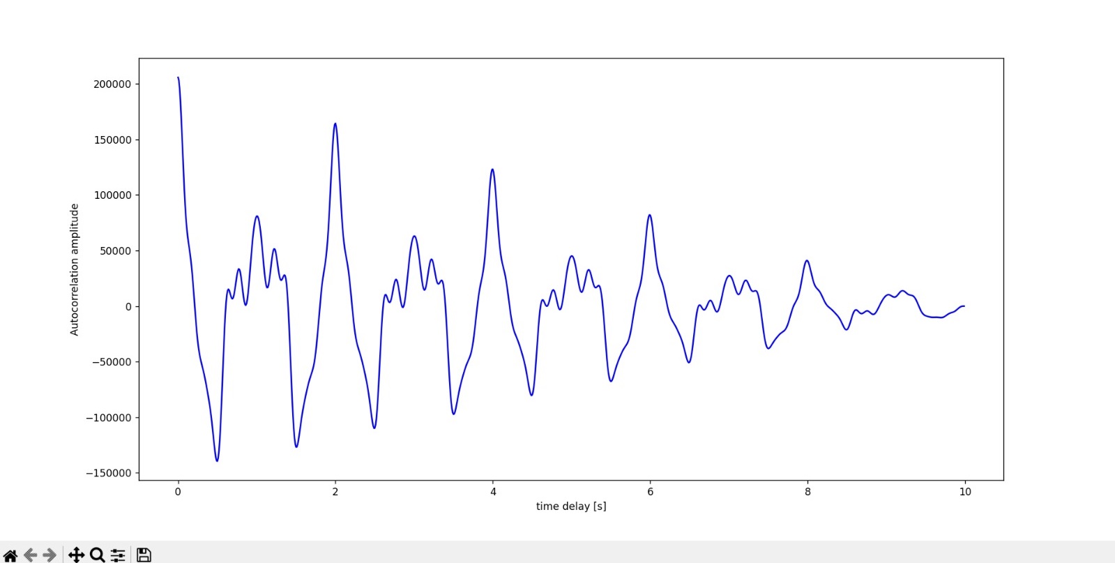
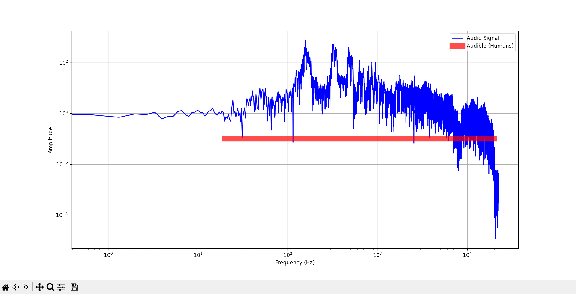
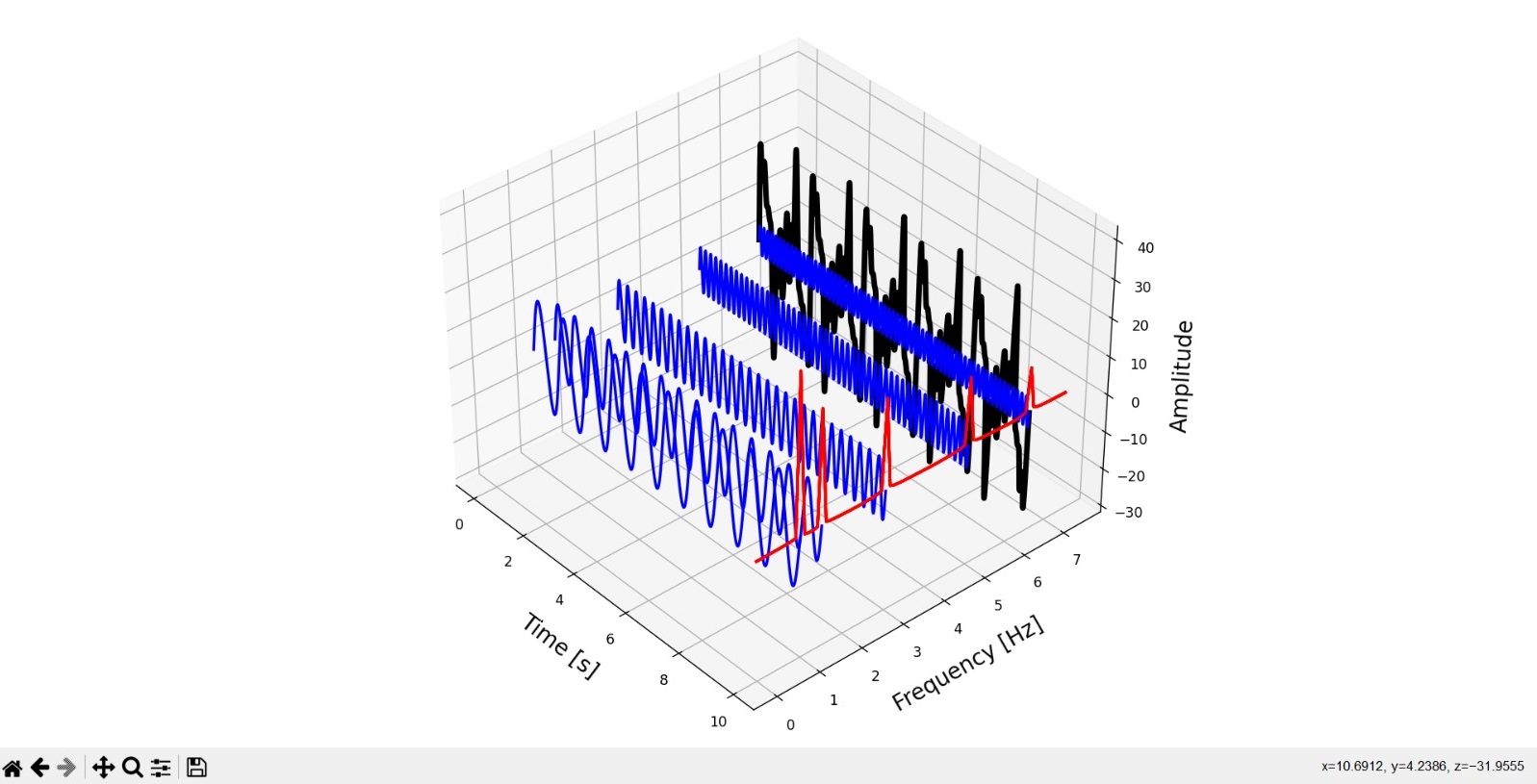
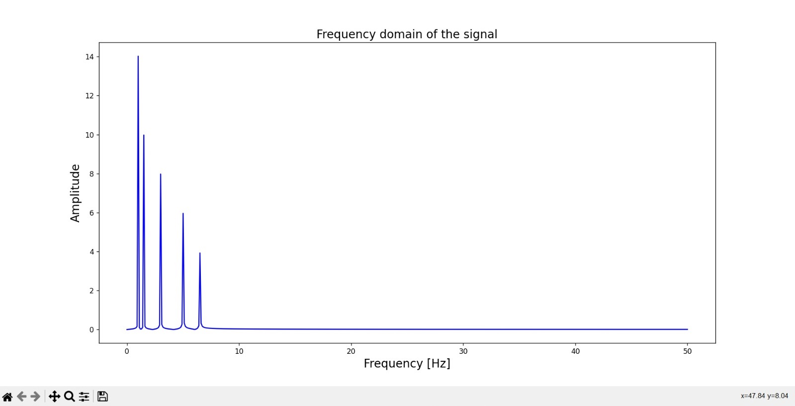
Transformation Between Time and Frequency Domains


Transformation Between Time and Frequency Domains Transformation Between Time and Frequency Domains Transformation Between Time and Frequency Domains

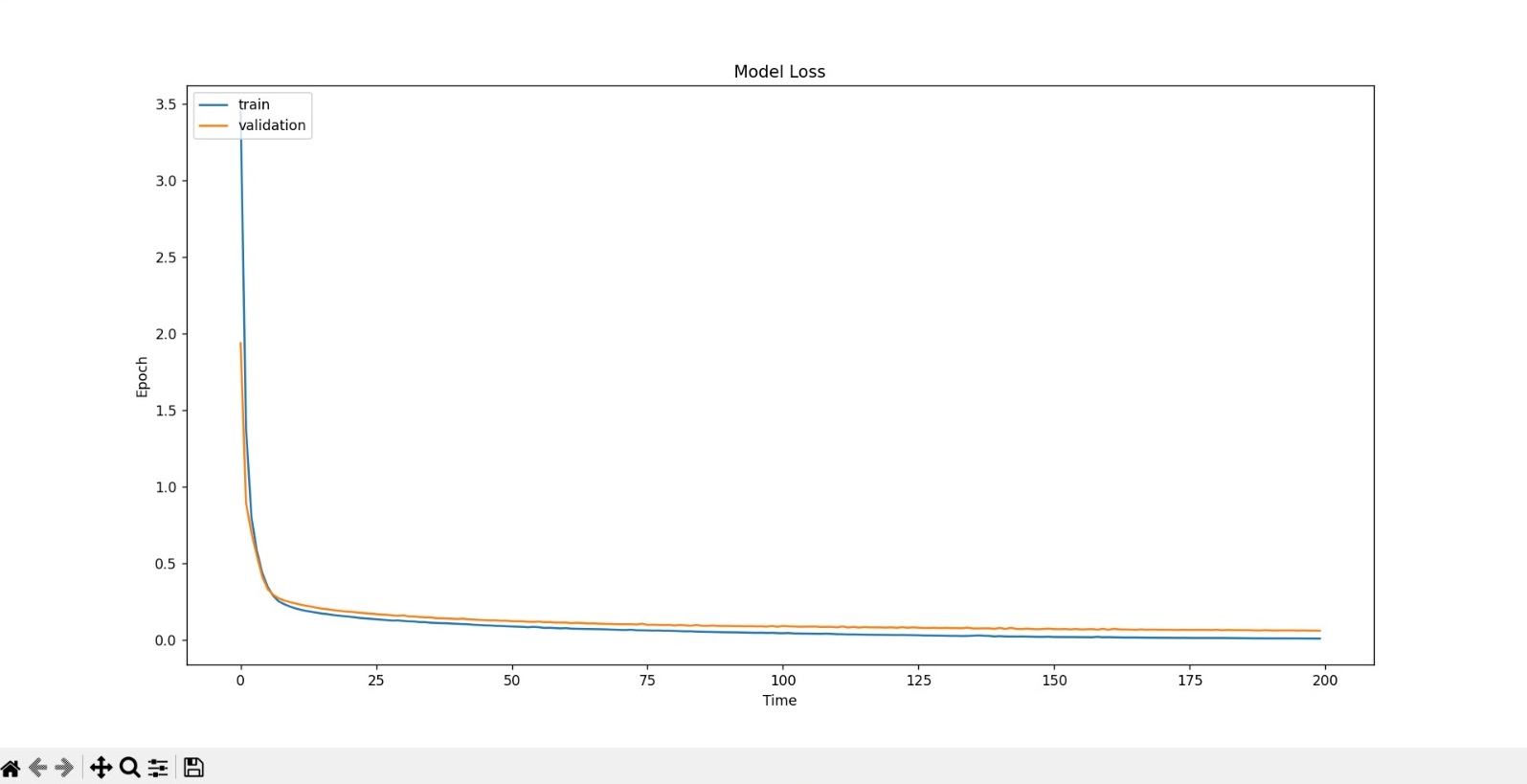
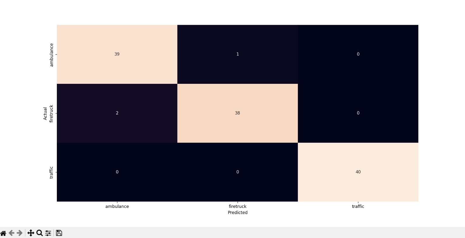
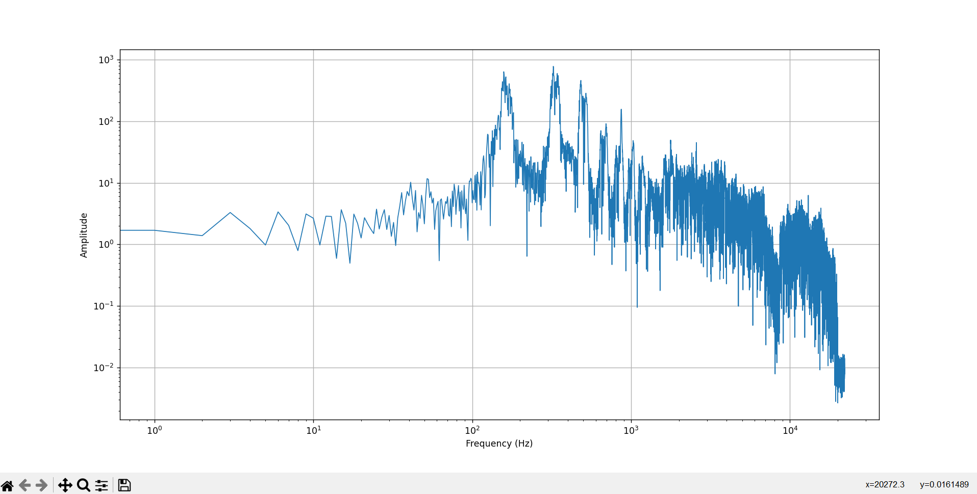
Emergency Vehicles Sound Classification


Emergency Vehicles Sound Classification Emergency Vehicles Sound Classification

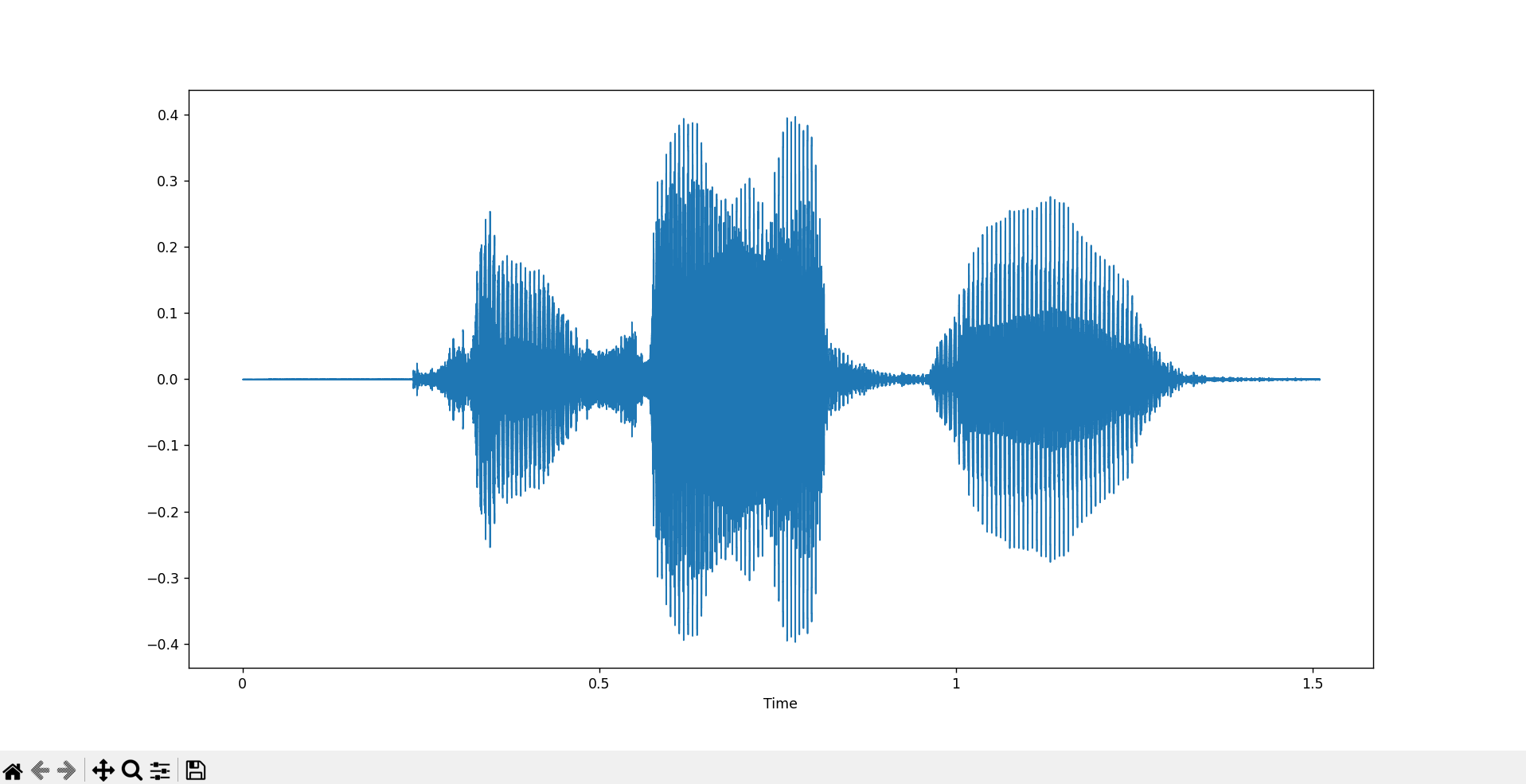
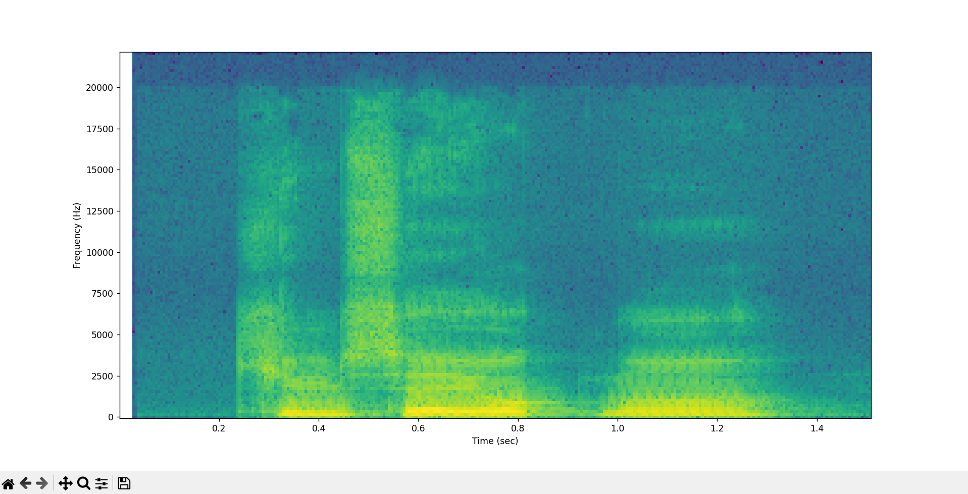
Human Sound Analysis


Human Sound Analysis Human Sound Analysis Human Sound Analysis Human Sound Analysis